Spatial data foundations for nature analysis
Exploring key concepts, standards, and libraries.
Welcome to the Nature Data Newsletter. Each month, we share insights with data enthusiasts, GIS experts, and investors learning about nature data.
We envision a world where large-scale data analysis improves the way we understand and value nature. This future drives Cecil’s mission to make nature data accessible.
Spatial data sit at the core of all nature analysis. An up-to-date understanding of spatial data is essential for any team working with nature data.
This newsletter continues our series on nature data workflows by focusing on foundational spatial data concepts, standards, and libraries. Starting here prepares us to move into deeper topics, such as spatial data indices and creating an Area of Interest (AOI) for analysis workflows.
Coordinate systems
Spatial data include numeric information that allows you to position the data somewhere on Earth. These numbers are part of a coordinate system that provides a frame of reference to locate features, join data, and tie analysis to a specific location.
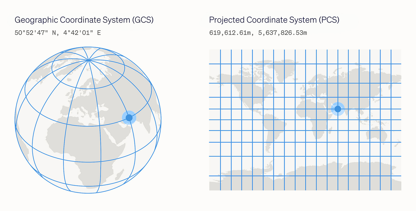
In nature data analysis, you'll encounter both Geographic Coordinate Systems and Projected Coordinate Systems. Below, we've provided a brief description of their use, their interaction, and considerations for their application.
Geographic Coordinate System
A Geographic Coordinate System uses a three-dimensional spherical or ellipsoid model of Earth’s surface - technically referred to as a ‘datum’ - to define locations on Earth. A point is referenced by its longitude and latitude values, which are angles measured from the Earth’s center to a point on the Earth’s surface. These angles are often measured in degrees.
There are many different datums, and therefore, many different Geographic Coordinate Systems. The World Geodetic System 1984 (WGS84) is a universal Geographic Coordinate System that is suitable for mapping global data. Another example is the Australian Geodetic Datum 1984, which is tailored to fit the Earth’s surface around Australia, providing high precision for this continent but lower accuracy elsewhere.
Projected Coordinate System
A Projected Coordinate System uses a two-dimensional Cartesian coordinate system to represent locations on Earth as a flat surface, such as a map or a computer screen.
In addition to defining a Geographic Coordinate System that models the Earth's surface, a Projected Coordinate System applies a map projection. This mathematical transformation adjusts geographic coordinates to account for Earth's curvature and projects them onto a flat surface. Numerous map projections exist, each minimising distortion over a specific area or for a particular purpose. For example, some map projections preserve accurate areas across all regions, while others maintain precise angles or distances.
Considerations for your nature data analysis workflow
Selecting or transforming a coordinate system
When selecting or transforming a coordinate system, it is important to consider the units and spatial extent of the data, geographic region, and total area you aim to analyse.
When you receive a dataset, it will likely come with an existing coordinate system. Therefore, it's important to understand how to transform it.
As an example of how this relates to a data analysis workflow, Snowflake refers to coordinate systems as a Spatial Reference System. The Geography data type in Snowflake uses WGS84 as a standard Geographic Coordinate System. By contrast, the Geometry data type enables users to specify a Projected Coordinate System. Users can specify the Spatial Reference System of data by assigning a spatial reference identifier, allowing for the most suitable coordinate system to be chosen for a specific region and use case.
Vector and raster data
The vast majority of nature data analysis will utilise a combination of both vector and raster data types. Sometimes, these data types are used together in a single workflow, while other times, separate workflows are developed for each.
Vector
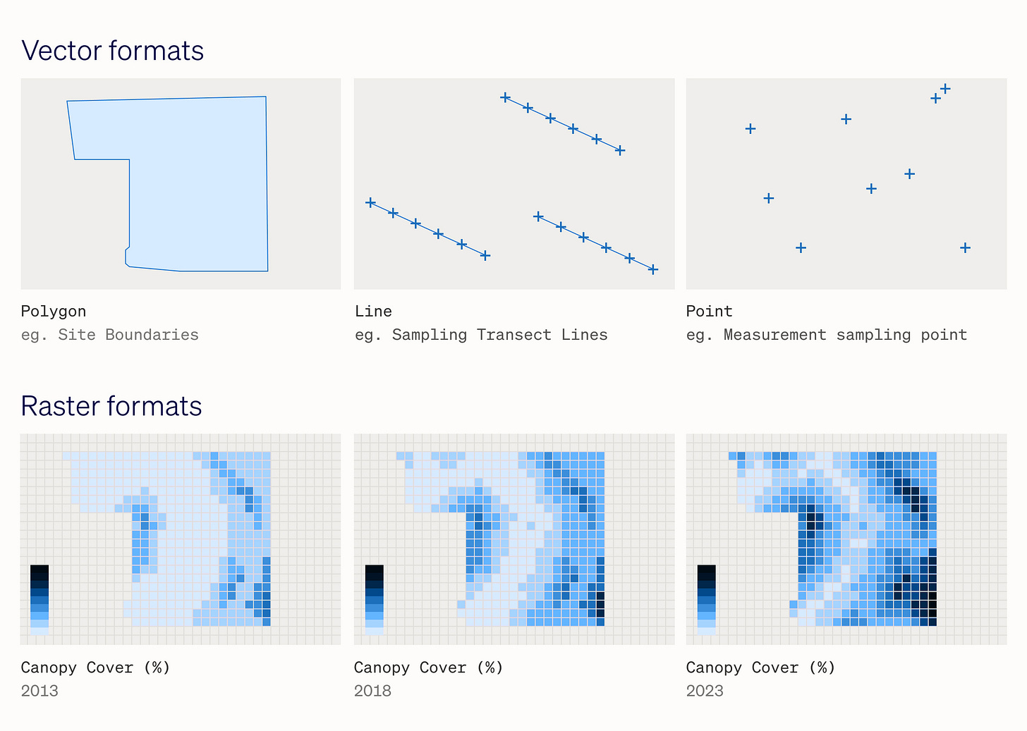
Vector data are lightweight data comprising individual points stored as coordinate pairs that indicate physical locations in the world. Vector data can take various forms: points, lines, or polygons.
In nature data analysis, vectors are typically used to represent features, such as site boundaries (polygons), sampling transect paths (lines), or measurement samples (points). Vector data representations are essential for defining an area of interest for specific data analysis workflows, such as a farm's property boundaries.
Raster
Raster data consists of a grid of pixels, with each pixel holding a specific value.
Raster data are usually used to represent continuous values, such as canopy cover, temperature, or rainfall. Categorical data, such as land cover class coverage, is often represented in raster format. Raster data is crucial in analysing nature data, as most remote sensing data is collected, stored, and delivered in this format.
Considerations for your nature data analysis workflow
Formats and storage
Vector and raster data are stored in many different formats that have been developed over several decades. Most formats were originally developed for specific software programs and optimised for data storage capacity. Recently, several initiatives have begun to support these data types on widely adopted cloud platforms.
Selection criteria
In a previous newsletter, we discussed how data format and storage should be considered when selecting nature datasets to use in your analysis workflow. We also created a criteria factsheet to support your next data search.
Formats, standards, and libraries
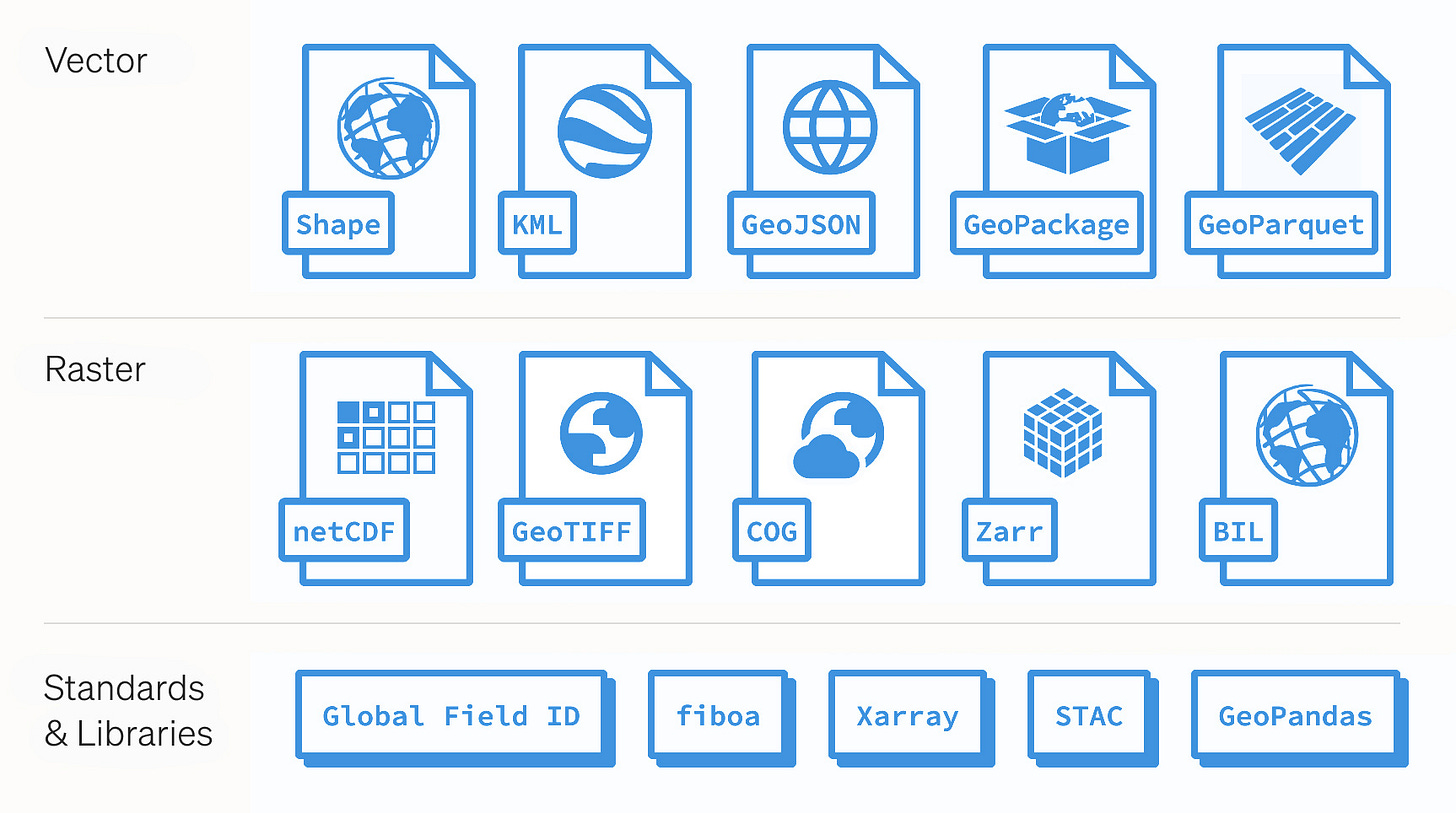
Below is a compiled list of common formats, standards, and libraries that you may encounter in your workflows with vector and raster data.
Vector
A shapefile is an Esri vector file format for storing the location, shape, and certain attributes of geographic features.
Keyhole Markup Language (KML) is an XML-based vector file format originally developed for Google Earth, but has since been widely adopted in the GIS ecosystem.
GeoJSON is an open standard vector file format based on JSON (JavaScript Object Notation). GeoJSONs are used in spatial data analysis to share areas of interest, such as property boundaries, in a machine readable format.
The GeoPackage encoding standard describes a set of conventions for storing vector data within a SQLite database.
GeoParquet is a column-oriented data format. GeoParquet is an Open Geospatial Consortium (OGC) standard that adds interoperable geospatial types (Point, Line, Polygon) to Parquet.
Raster
NetCDF (Network Common Data Form) is a set of software libraries and machine-independent data formats that supports the creation, access, and sharing of array-oriented scientific data.
GeoTIFF and Cloud Optimised GeoTIFF
GeoTIFF and Cloud Optimised GeoTIFF (COG) are a widely adopted metadata standard that enables georeferencing information to be embedded within a raster file.
Zarr is a community project aimed at developing specifications and software for storage of large N-dimensional typed arrays.
Developed by Esri, Band interleaved by Line (BIL), Band interleaved by Pixel (BIP), and Band Sequential (BSQ) are three common methods of organizing image data for multiband images.
Standards and libraries
After ingesting and validating field boundaries, Global FieldID assigns a unique alphanumeric code to each field enabling field identification of agricultural land plots, globally.
Fiboa (Field Boundaries for Agriculture) is a new collaborative project focused on improving the interoperability of farm field boundary data by representing them in GeoJSON & GeoParquet in a standardised way.
Xarray provides data models for working with labeled arrays and datasets.
The STAC specification is a common language to describe geospatial information so that it can more easily be worked with, indexed, and discovered.
GeoPandas is an open source project to make working with geospatial data in Python easier.
We'd love to hear from anyone working with these different spatial data standards and formats to analyse nature data – drop us a line at hello@cecil.earth.
This is the second newsletter in a series focusing on nature data workflows. In the next issue, we'll delve into creating Areas of Interest (AOIs) for detailed asset-level analysis, discuss spatial indexes like H3, and examine how these advancements contribute to positive action for nature.
Early User Testing Program
Support Cecil’s mission to make nature data accessible by joining our Early User Testing Program.
We are seeking individuals with diverse data skills (such as Python, SQL, and GIS) to test a range of nature data analysis workflows on our platform.
Notices
BloomLabs explore whether biodiversity credits are assets or commodities.
Chloris Geospatial welcomes the Cisco Foundation and NextSTEP as new investors.
Nature-Tech Memos publish a weekly newsletter on the latest and greatest in Nature Tech and Nature Finance.
Planet record Forest Carbon Planetary Variable webinar to discuss their accurate estimates of measurements of the aboveground carbon stored in forests.
Space Intelligence release a series of webinars on ways project developers and investors are using land cover data to maximise nature impact.
The World Economic Forum explore how direct biomass estimation can improve forest carbon accounting.
Thank you
A special thank you to everyone who supported us this month with feedback, introductions, and advice:
Andrew Farnsworth, Chris Holmes, Claudia Röösli, Claire Wightman, Daniel Osgood, David Marvin, Edmund Pragnell, Franziska Schrodt, Felix Morsdorf, Gabi Ceregra, Isabelle Helfenstein, Jochem Braakhekke, Karl Burkart, Luc Sierro, Marius Vögtli, Merry Schuman, Niki Lewis, Nkwi Flores, Ryan Abernathey, and Steve Toben.
Keep reading
This newsletter is created by Cecil. From curating data providers, to preparing data for analysis, Cecil’s nature data infrastructure helps teams access accurate and precise nature data. They are trusted by companies such as Foresight Sustainable Forestry, Kilter Rural, and Impact Ag Partners to manage data on 3,000+ natural assets and 3+ million hectares.
Enjoy the newsletter? Please forward to a friend.


