Exploring spatial indexes
Challenges in scaling nature data analysis and how spatial indexes might help.
Welcome to the Nature Data Newsletter. Each month, we share insights with data enthusiasts, GIS experts, and investors learning about nature data.
Last month, we introduced the foundations of spatial data - a starting point for anyone with a nature data workflow. We discussed spatial data standards, libraries and formats commonly adopted across the nature data community.
This newsletter continues our series on nature data analysis workflows by focusing on spatial indexes. We explore common challenges caused by the increased scale and complexity of nature datasets and introduce spatial indexes as a possible solution.
Datasets are getting larger and more complex
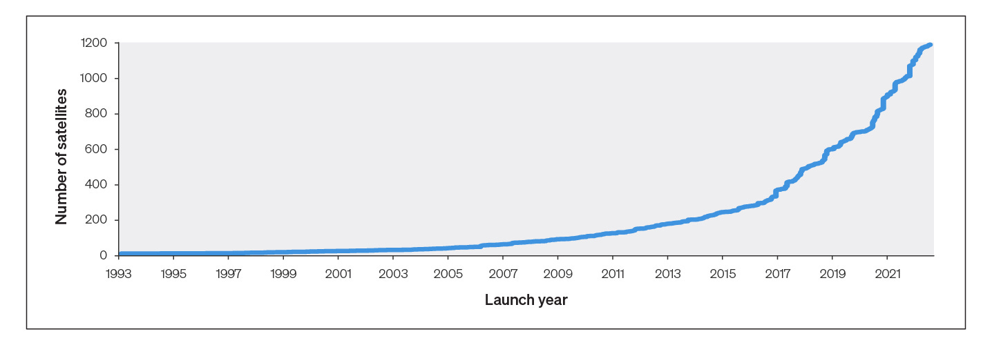
Advanced measurement technologies like remote sensing satellites have greatly increased the amount of spatial data generated about nature. In 2023, over 100 TB of satellite imagery was collected daily, and an additional 20,000 satellites are predicted to be deployed by 2030. This growth is paired with the emergence of new data collection technologies such as hyperspectral sensors, camera traps, and bioacoustic devices.
Such large volumes of data are creating processing and analysis challenges for teams with raster-based nature data workflows:
Computation
Large datasets often exceed the capacity of file-based tools. In our research with over 30 subject matter experts, we found that storage or processing limitations slowed down raster-based analysis tasks - especially when working with many variables at high spatial or temporal resolutions.
"When conducting nature analysis at a continental scale, I'm often forced to downscale due to computational limits. These limitations affect other analysis decisions, such as the resolution I can work with."
Joining data
There are a range of parameters to consider when joining raster data from different sources, including the coordinate reference system (CRS), bounding box and spatial resolution. There is no industry standard for setting these parameters, so data teams must manually transform rasters from different sources in order to combine them in an analysis.
CRS selection
The right choice of CRS for a raster is important to accurately represent areas (e.g. farm boundaries), distances (e.g. bird migrations), or to compare sites across large areas (e.g. N. America). For instance, the global CRS EPSG 4326 is not an equal-area grid: on the equator, one degree of longitude is the same as one degree of latitude, but one degree of longitude becomes a smaller absolute distance as you move away from the equator. This means that sites in high latitude regions are represented less accurately by EPSG 4326 than those in the tropics.
If you’re looking for an introduction to coordinate systems, have a look at our newsletter on spatial data foundations.
After hearing from many experts and data teams about these emerging challenges, we decided to explore spatial indexes as a solution.
What are spatial indexes?
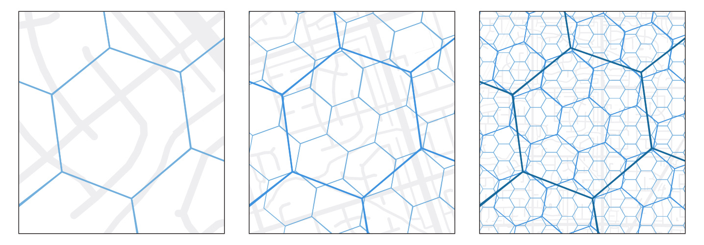
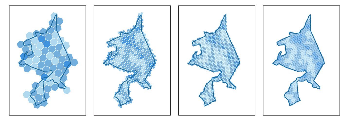
Spatial indexes, also referred to as Discrete Global Grid Systems (DGGS), are grid systems that organise spatial data into a discrete grid of cells with a unique identifier (index) that locates their position on Earth. Think of cells as pixels with a pre-defined size, shape and location that are shared between all datasets that use them. Cells must be a shape that can tesselate on a grid, such as a square, hexagon or triangle, so that no space is missed on the Earth’s surface. Grids are also usually hierarchical, in that they have multiple resolutions where higher resolution grids (with more cells) are nested within the cells of lower resolution grids. Since all cells have a unique ID, data teams can use spatial indexes to convert any raster grid onto a universal index, which can be used to easily combine data from many different data sources.
Common spatial indexes
Different spatial indexes have their own unique characteristics, usage scenarios and benefits. Below we explore two common spatial indexes – H3 and S2.
H3
H3 is a spatial index developed by Uber for the purpose of visualising and exploring spatial data patterns, such as distances and route finding.
H3 was designed to use hexagons because they are the closest tessellating shape to a circle. This makes them effective at representing distances between neighboring cells. A grid of hexagons also captures curved lines better than a grid of squares.
H3 is a hierarchical system with 16 nested resolutions. Indexing spatial data at a given resolution returns a list of one or more cell IDs that cover the whole area represented. For reference, a H3 cell at resolution 15 is approximately 0.9 m² (see here for more details about H3 resolutions). Converting between H3 resolutions is straightforward, but is imperfect because a hexagon at one resolution cannot be entirely filled by hexagons at a higher resolution.
H3 suffers from low area distortion (at the highest resolution, cells vary from 0.54 m² to 1.08 m² globally). However, cell areas still vary a little because the H3 system maps the grid onto an icosahedron rather than a sphere.
S2
S2 is a spatial index developed by Google to work with spherical projections. Unlike traditional geographic information systems, which represent data as flat two-dimensional projections (similar to an atlas), S2 represents all data on a three-dimensional sphere (like the globe).
S2 is made up of approximate squares, with the lowest resolution being the six faces of a cube projected onto the Earth’s spherical surface. Higher resolutions are then created by subdividing lower resolution cells into four.
As a grid of squares, S2 is not as good at preserving neighborhood relationships and curved lines as the hexagons of H3. However, S2 cells are perfectly nested between resolutions, meaning a cell at one resolution is entirely captured by four cells at the next resolution. S2 cells also suffer from less area distortion at the poles due to their spherical projection, although H3 cells are more uniform in size than S2 cells when considering the entire globe.
Using spatial indexes in nature data workflows
Spatial indexes have become increasingly popular in nature data workflows because of their ability to represent large volumes of data as a table of standardised cell IDs. However, these efficiency gains can also compromise accuracy for certain use cases. A thriving community of builders is working on fully understanding different trade-offs and building tools that overcome these challenges. As it stands, there are some considerations for using spatial indexes in nature data workflows:
Computation
Transforming raster or vector data into a spatial index can optimise it for certain data operations. However, the computational advantages of spatial indexes depend on the type of index. For example, H3 improves the efficiency of area and distance calculations. On the other hand, many existing spatial analysis libraries are designed to run on rasters and would either be slower or not work at all with a spatial index like H3.
Joining data
Spatial data is generated about a specific region with a specific CRS, bounding box, pixel grid and resolution, making it impossible to combine datasets without pre-processing. Transforming multiple rasters and vectors into spatial indexes standardises them into the same structure with identical cell references, making them immediately consistent and joinable.
Resolution
Spatial indexes usually have a resolution cap. This means they might not be suitable for analyses requiring extremely high precision (e.g., < 1 m²). H3 also has imperfect child containment between resolutions. As you increase H3 resolution, the cells at that resolution do not nest perfectly within those of the lower resolution.
Representing complex geometries
Spatial indexes might not accurately depict the exact spatial coverage of complex polygons and lines. For instance, the hexagons of H3 are better at representing curved lines than the squares of S2. However, S2 is better at representing straight lines running in cardinal directions (i.e., N, E, S, or W).
Data loss
Converting from a raster to a spatial index involves some data loss. For instance, if you convert from a raster to a spatial index and then back to a raster, you won't get the same raster you started with. This effect isn't unique to spatial indexes. There will also be data loss whenever you convert spatial data from one CRS or resolution to another.
Notices
Cecil are bringing London's nature data community together to geek out over dumplings and cocktails on Thursday 25th July. RSVP here.
Chloris Geospatial share thoughts on the role of tech innovation in scaling up private financing of natural climate solutions.
Kanop is looking for a Chief Science & Policy Officer who could join the team as a Co-founder. Please email romain.fau@kanop.io for more details.
Renoster launch REDD: Neutral’s high-integrity, transparent market for REDD+ projects to address long-standing challenges in the REDD+ credit market.
Thank yous
A special thank you to everyone who supported us this month with feedback, introductions, and advice:
Ali Swanson, Alex Burns, Ben Harries, Claire Wightman, David LeBauer, Fernando Mateos González, Mary Jane Wilder, Natasha Batista, Nitin Magima, Matthias Asemota, Maryn van der Laarse, Miguel Fernandez, Roberto Miethe, Steven Cramer, and Wade Cooper.
Keep reading
Sponsorship
Do you want to share monthly updates with our engaged audience of 1500+ nature data users and investors? Please contact rory@cecil.earth to find out more about our newsletter sponsorship packages.
This newsletter is curated by Cecil, a team on a mission to make nature data accessible. Their platform helps data teams access analysis-ready commercial and public nature datasets, eliminating the need for cleaning, harmonising, and pre-processing tasks. Whilst currently focused on aboveground biomass, they will soon launch land cover and land use datasets to support market-leading nature-tech applications, consultants, and nature restoration professionals.
Enjoy the newsletter? Please forward to a friend.


